BIOLOGY FOR LIFE
  • IB Bio Syllabus
    • Unity and Diversity (A) >
      • A1 molecules >
        • A1.1: Water
        • A1.2: Nucleic Acids
      • A2 Cells >
        • A2.1: Origins of Cells
        • A2.2: Cell Structure
        • A2.3: Viruses
      • A3 Organisms >
        • A3.1: Diversity of Organisms
        • A3.2: Classification and Cladistics
      • A4 Ecosystems >
        • A4.1: Evolution and Speciation
        • A4.2: Conservation of Biodiversity
    • Form and Function (B) >
      • B1 Molecules >
        • B1.1: Carbohydrates and Lipids
        • B1.2: Proteins
      • B2 Cells >
        • B2.1 Membranes and Membrane Transport
        • B2.2 Organelles and Compartmentalization
        • B2.3 Cell Specialization
      • B3 Organisms >
        • B3.1 Gas Exchange
        • B3.2 Transport
        • B3.3 Muscle and Motility
      • B4 Ecosystems >
        • B4.1 Adaptation to Environment
        • B4.2 Ecological Niches
    • Interaction and Interdependence (C) >
      • C1 Molecules >
        • C1.1: Enzymes and Metabolism
        • C1.2: Cell Respiration
        • C1.3: Photosynthesis
      • C2 Cells >
        • C2.1: Chemical Signaling
        • C2.2: Neural Signaling
      • C3 Organisms >
        • C3.1: Integration of Body Systems
        • C3.2: Defense Against Disease
      • C4 Ecosystems >
        • C4.1 Populations and Communities
        • C4.2 Transfers of Energy and Matter
    • Continuity and Change (D) >
      • D1 Molecules >
        • D1.1: DNA Replication
        • D1.2: Protein Synthesis
        • D1.3: Mutation and Gene Editing
      • D2 Cells >
        • D2.1: Cell and Nuclear Division
        • D2.2: Gene Expression
        • D2.3: Water Potential
      • D3 Organisms >
        • D3.1: Reproduction
        • D3.2: Inheritance
        • D3.3: Homeostasis
      • D4 Ecosystems >
        • D4.1: Natural Selection
        • D4.2: Stability and Change
        • D4.3: Climate Change
  • IB Requirements
    • Internal Assessment >
      • Research Design
      • Analysis
      • Conclusion
      • Evaluation
    • External Assessment >
      • Exam Revision
    • Extended Essay
    • Reflective Project
    • Collaborative Sciences Project
    • Learner Profile
  • Skills for Biology
    • Tools >
      • Experimental Techniques >
        • Addressing Safety
        • Measuring Variables >
          • Measurement Uncertainties
          • Observations
          • Biological Drawings
        • Applying Techniques >
          • Microscopy
      • Technology >
        • Tech to Collect Data
        • Tech to Process Data
      • Mathematics >
        • General Math
        • Units and Symbols
        • Processing Uncertainties
        • Graphing >
          • Types of Graphs
          • How to Graph
          • Graph Error Bars
    • Inquiry Processes >
      • Exploring >
        • Research Questions
        • Hypotheses and Predictions
      • Designing >
        • Variables
        • Sampling
      • Control of Variables
      • Collecting Data >
        • Data Tables
      • Processing Data
      • Interpreting Results
      • Concluding
      • Evaluating >
        • Error Analysis
  • Statistics
    • Descriptive Statistics >
      • Skew and the Normal Distribution
      • Outliers
      • Measures of Central Tendancy
      • Measures of Dispersion
      • Correlation Coefficients
      • Coefficient of Determination
    • Inferential Statistics >
      • Standard Error
      • T-Test
      • ANOVA
      • Kruskal-Wallis
      • X2 Test of Independence
      • X2 Goodness of Fit
    • Glossary of Statistic Terms and Equations
  • SHS Course Info
    • Above & Beyond >
      • Biology Club
      • Pumpkin Carving
      • Scavenger Hunt
      • Science News
      • Wood Duck Project (legacy)
      • Invasive Crayfish Project (legacy)
    • Assessment >
      • Class Grading IB Bio I
      • Class Grading IB Bio II
      • Daily Quizzes (legacy)
      • Lab Practicals (legacy)
    • Class Photos
    • Recommendations
  • Contact
    • About >
      • Philosophy
      • Resume
      • Reflection
      • Favorite Quotes
      • AEF Blog
  • Expeditions
    • Bahamas (2009)
    • Trinidad (2010)
    • Trinidad (2011)
    • Ecuador (2012)
    • Trinidad (2013)
    • Peru (2014)
    • Bahamas (2015)
    • Peru (2016)
    • Costa Rica (2017)
    • Costa Rica (2018)
    • Arizona (2022)
    • Florida (2023)
    • Belize (2024)
    • Costa Rica (2025)
  • Summer Ecology Research
  • Teacher Resources

Chi-Square (X2) Goodness of Fit
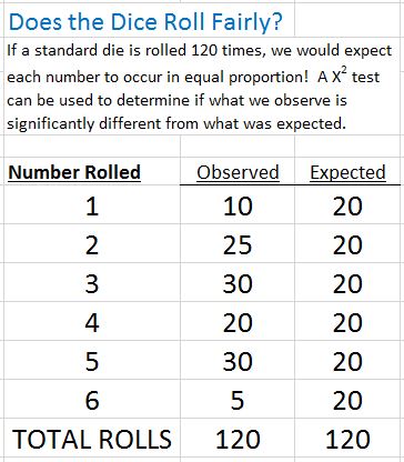
The chi-square (χ²) goodness of fit test is an inferential statistical tool used to determine whether observed experimental results match what would be expected based on a particular hypothesis or theoretical model. The χ² statistic is a single number that tells you how much difference exists between your observed counts and the counts you would expect in the population.  A low value for chi-square means there is little difference between what was observed and what would be expected.  In theory, if your observed and expected values were equal (“no difference”) then chi-square would be zero.  

“Chi” (χ) is a Greek letter andis pronounced as “kai” (not “chee”).  The following are χ2 test criteria that must be met for validity.
  • The χ2 test should only be used with counts or frequencies (it is, therefore, not suitable for measurements).
  • It should not be used with derived values (such as a percentage or density derived from counts).
  • The χ2 test should be used to compare a set of observed (experimental) results to a set of expected or theoretical results.
  • The minimum sample size should be 20 (n = 20). This statistical test is invalid when sample sizes are too small. Larger samples are likely to yield greater significance. 
  • This statistical tool is not valid if any of the categories has a frequency of 0 (0 counts).
  • Students must be able to group the data into distinct/discrete categories (such as “a” or “b”).

Genetic crosses and inheritance patterns represent the most common application of the chi-square (χ²) goodness of fit test in IB Biology coursework. When you cross two organisms and count the offspring phenotypes, you can use chi-square to test whether your results match expected Mendelian ratios like 3:1 or 9:3:3:1. The test helps you determine if any deviations from expected ratios are due to random chance or indicate that something else might be influencing inheritance patterns. You might also apply this test to analyze population genetics data, such as testing whether allele frequencies in a population match Hardy-Weinberg expectations, or examining ecological data like species distribution patterns.

Tip: The Chi-square statistic can only be used on numbers. They can’t be used for percentages, proportions, means or similar statistical value. For example, if you have 10 percent of 200 people, you would need to convert that to a number (20) before you can run a test statistic.
Just like other statistical tests, the Chi-Square Goodness of Fit tests two hypotheses.  
Null Hypothesis (Ho):
"There is not a significant difference between what was observed and what was expected; any difference between observed and expected is likely due to chance and sampling error."

For example:  
  • There is no significant difference between the phenotypes of the offspring as expected by the Punnett grid and the observed phenotypes in the offspring; any differences seen between observed and expected numbers may be due to chance or sampling error.
Alternative Hypothesis (H1):
"There is a significant difference between what was observed and what was expected; the differences between observed and expected is likely not due to chance or sampling error."

For example:  
  • There is a significant difference between the phenotypes of the offspring as expected by the Punnett grid and the observed phenotypes in the offspring; the differences seen between observed and expected numbers are likely not due to chance or sampling error.

How to Calculate a Chi-Square Goodness of Fit

​Computing the chi-square statistic involves using the formula χ² = Σ[(observed - expected)²/expected] for each category, then summing all values. 
Picture
  1. The first step in the calculation of an X2 value is to determine the expected numbers.  In genetics, you'd use a Punnett square to determine the theoretical expected values. ​
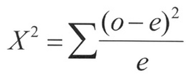
  2. Then, use the formula for each observed and expected category: (O-E)2 / E
  3. The results are added together to get a final X2 value.  
  4. ​The calculated X2 value is than compared to the “critical value  X2” found in an X2 distribution table.  

You'll then determine your degrees of freedom (number of categories minus 1) and compare your calculated χ² value to the critical value from a chi-square table at your chosen significance level (typically p = 0.05).
  • The X2 distribution table represents a theoretical curve of  expected results. ​The expected results are based on DEGREES OF  FREEDOM.  Degrees of Freedom = number of categories – 1. ​
  • ​​The X2 distribution table is organized by the Level of  Significance.  The level of significance is the maximum tolerable probability of accepting a false null hypothesis.  We use 0.05.  
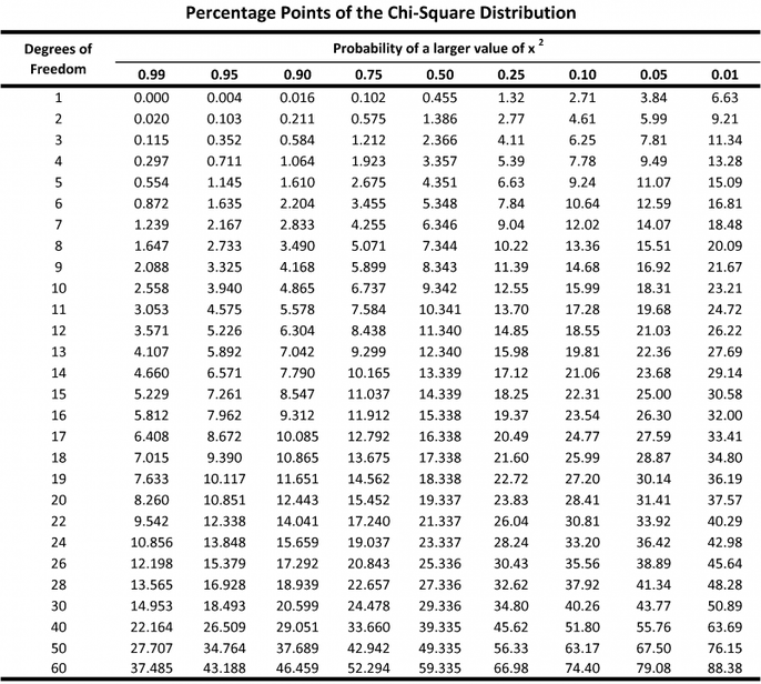
Picture
​Understanding what your results mean is crucial for drawing valid biological conclusions. 
  • If the calculated value is lower than the critical value in the table at the 0.05 level of significance, accept the null hypothesis. The chi-square suggests that the observed data fits the expected pattern well enough that any differences could be due to random sampling variation. 
  • If the calculated value is higher than the critical value in the table at the 0.05 level of significance, reject the null hypothesis.  The chi-square suggests that the deviation from expected results is too large to be explained by chance alone. 
Drawing biological significance from statistical results requires careful consideration of what rejection or acceptance means in your specific context. Rejecting the null hypothesis doesn't automatically mean the expected values are wrong; factors like sample size or uncontrolled environmental influences may be affecting the results. 

Performing a Chi-Square test in Google Sheets

  • The formula to  use is =CHITEST(observed_range, expected_range).  Where "observed_range" is the counts associated with each category of data and "expected_range" is the expected counts for each category under the null hypothesis.

Performing a Chi-Square test in Excel 

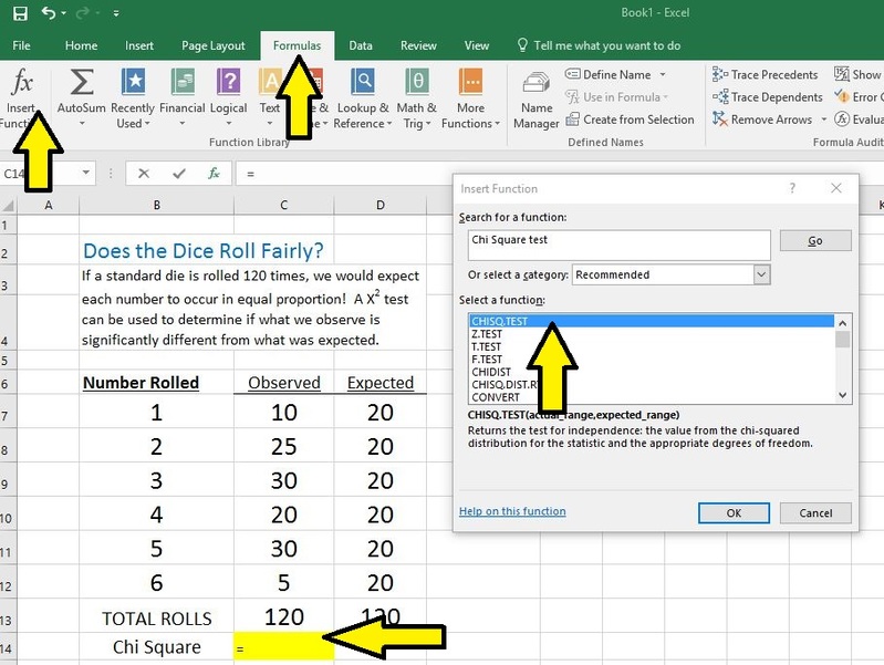
  • ​Enter your observed and expected values in columns.
  • Click the box in which you want the Chi Square value to be placed
  • Select Insert Function from the Formulas tab
  • Search for Chi Square test and select the CHISQ.TEST from the menu
  • Hit OK
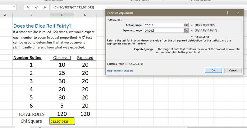
  • Select all of your observed (actual) results for the Actual_range and all of your expected results for the Expected_range.
  • Hit OK
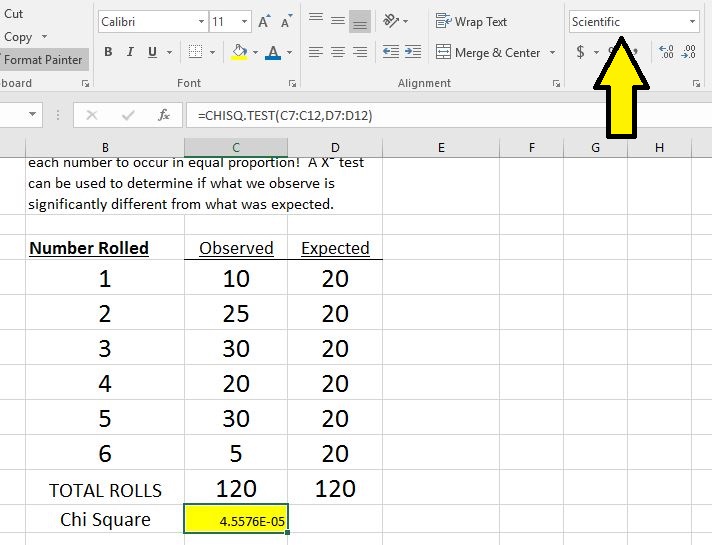
  • The resulting value is the P value for the Chi-Square  test.  If you don't want it to be in scientific notation, you can change the format of the number by selecting "number"  instead of "scientific."
  • If the p-value you get is less than 0.05, reject the null hypothesis  and conclude that there is a significant difference between the observed and expected values.  Likewise, if the p-value is more than 0.05, accept the null hypothesis and conclude that there is no significance difference between the observed and expected. ​
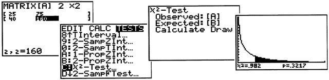
I give many of my IB Biology resources away, for the benefit of students and teachers around the world. 
If you've found the materials helpful, please consider sending a gift from our classroom wish list.


​Did I forget something?  Know of a mistake? Have a suggestion?  Let me know by emailing me here.

Before using any of the files available on this site,
​please familiarize yourself with the 
Creative Commons Attribution License. 
​​​It prohibits the use of any material on this site for commercial  purposes of any kind.  ​
​
Picture
  • IB Bio Syllabus
    • Unity and Diversity (A) >
      • A1 molecules >
        • A1.1: Water
        • A1.2: Nucleic Acids
      • A2 Cells >
        • A2.1: Origins of Cells
        • A2.2: Cell Structure
        • A2.3: Viruses
      • A3 Organisms >
        • A3.1: Diversity of Organisms
        • A3.2: Classification and Cladistics
      • A4 Ecosystems >
        • A4.1: Evolution and Speciation
        • A4.2: Conservation of Biodiversity
    • Form and Function (B) >
      • B1 Molecules >
        • B1.1: Carbohydrates and Lipids
        • B1.2: Proteins
      • B2 Cells >
        • B2.1 Membranes and Membrane Transport
        • B2.2 Organelles and Compartmentalization
        • B2.3 Cell Specialization
      • B3 Organisms >
        • B3.1 Gas Exchange
        • B3.2 Transport
        • B3.3 Muscle and Motility
      • B4 Ecosystems >
        • B4.1 Adaptation to Environment
        • B4.2 Ecological Niches
    • Interaction and Interdependence (C) >
      • C1 Molecules >
        • C1.1: Enzymes and Metabolism
        • C1.2: Cell Respiration
        • C1.3: Photosynthesis
      • C2 Cells >
        • C2.1: Chemical Signaling
        • C2.2: Neural Signaling
      • C3 Organisms >
        • C3.1: Integration of Body Systems
        • C3.2: Defense Against Disease
      • C4 Ecosystems >
        • C4.1 Populations and Communities
        • C4.2 Transfers of Energy and Matter
    • Continuity and Change (D) >
      • D1 Molecules >
        • D1.1: DNA Replication
        • D1.2: Protein Synthesis
        • D1.3: Mutation and Gene Editing
      • D2 Cells >
        • D2.1: Cell and Nuclear Division
        • D2.2: Gene Expression
        • D2.3: Water Potential
      • D3 Organisms >
        • D3.1: Reproduction
        • D3.2: Inheritance
        • D3.3: Homeostasis
      • D4 Ecosystems >
        • D4.1: Natural Selection
        • D4.2: Stability and Change
        • D4.3: Climate Change
  • IB Requirements
    • Internal Assessment >
      • Research Design
      • Analysis
      • Conclusion
      • Evaluation
    • External Assessment >
      • Exam Revision
    • Extended Essay
    • Reflective Project
    • Collaborative Sciences Project
    • Learner Profile
  • Skills for Biology
    • Tools >
      • Experimental Techniques >
        • Addressing Safety
        • Measuring Variables >
          • Measurement Uncertainties
          • Observations
          • Biological Drawings
        • Applying Techniques >
          • Microscopy
      • Technology >
        • Tech to Collect Data
        • Tech to Process Data
      • Mathematics >
        • General Math
        • Units and Symbols
        • Processing Uncertainties
        • Graphing >
          • Types of Graphs
          • How to Graph
          • Graph Error Bars
    • Inquiry Processes >
      • Exploring >
        • Research Questions
        • Hypotheses and Predictions
      • Designing >
        • Variables
        • Sampling
      • Control of Variables
      • Collecting Data >
        • Data Tables
      • Processing Data
      • Interpreting Results
      • Concluding
      • Evaluating >
        • Error Analysis
  • Statistics
    • Descriptive Statistics >
      • Skew and the Normal Distribution
      • Outliers
      • Measures of Central Tendancy
      • Measures of Dispersion
      • Correlation Coefficients
      • Coefficient of Determination
    • Inferential Statistics >
      • Standard Error
      • T-Test
      • ANOVA
      • Kruskal-Wallis
      • X2 Test of Independence
      • X2 Goodness of Fit
    • Glossary of Statistic Terms and Equations
  • SHS Course Info
    • Above & Beyond >
      • Biology Club
      • Pumpkin Carving
      • Scavenger Hunt
      • Science News
      • Wood Duck Project (legacy)
      • Invasive Crayfish Project (legacy)
    • Assessment >
      • Class Grading IB Bio I
      • Class Grading IB Bio II
      • Daily Quizzes (legacy)
      • Lab Practicals (legacy)
    • Class Photos
    • Recommendations
  • Contact
    • About >
      • Philosophy
      • Resume
      • Reflection
      • Favorite Quotes
      • AEF Blog
  • Expeditions
    • Bahamas (2009)
    • Trinidad (2010)
    • Trinidad (2011)
    • Ecuador (2012)
    • Trinidad (2013)
    • Peru (2014)
    • Bahamas (2015)
    • Peru (2016)
    • Costa Rica (2017)
    • Costa Rica (2018)
    • Arizona (2022)
    • Florida (2023)
    • Belize (2024)
    • Costa Rica (2025)
  • Summer Ecology Research
  • Teacher Resources