Chi-Square (X2) Test for Independence 

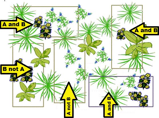
Chi-square Test for Independence is a statistical test commonly used to determine if there is a significant association between two variables.  For example, a biologist might want to determine if two species of organisms associate (are found together) in a community. 

Does Species A associate with Species B?

Species A

Species B

Just like other statistical tests, the Chi-Square Test for Independence tests two hypotheses:

Null Hypothesis:
"There is not a significant association between variables, the variables are independent of each other; any association between variables is likely due to chance and sampling error."

For example:  

• There is no significant association between Species A and Species B; the species are independent of each other.  The location of Species A has no effect on the location of Species B.

Alternative Hypothesis:
"There is a significant (positive or negative) association between variables; the association between variables is likely not due to chance or sampling error."

For example:  

• There is a significant association between Species A and Species B; the species are dependent.  Either Species A significantly associates with Species B or Species A does not significantly associate with Species B.

How to Calculate a Chi-Square Test of Independence

The first step is to collect raw data for the occurrence of each variable.  This is often done via random sampling using a quadrant.  In our example, there are five quadrants.  Determine: 

• The number of quadrants with both species present
• The number of quadrants with Species A but not Species B
• The number of quadrants with Species B but not Species A
• The number of quadrants with neither species 

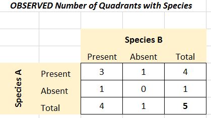
Then create a "contingency table" to display your results.  In the Chi-Square test, these are your OBSERVED values.

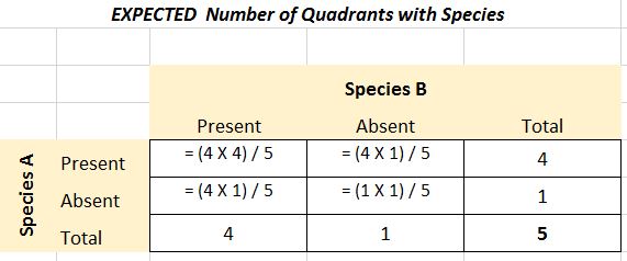
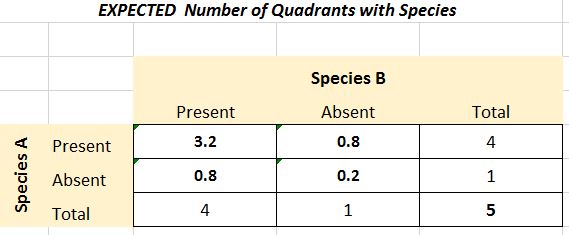
Next you need to determine what would be EXPECTED assuming the species are randomly distributed with respect to each other.   Expected frequencies = (row total X column total) / grand total

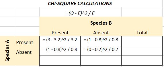
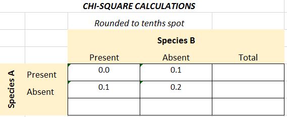
Now that you have OBSERVED and EXPECTED values, apply the Chi-Square formula in each part of the contingency table by determining (O-E)2 / E for each box.

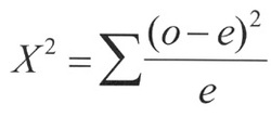
The final calculated chi-square value is determined by summing the values:

• X2 = 0.0 + 0.1 = 0.1 + 0.2 = 0.4

---

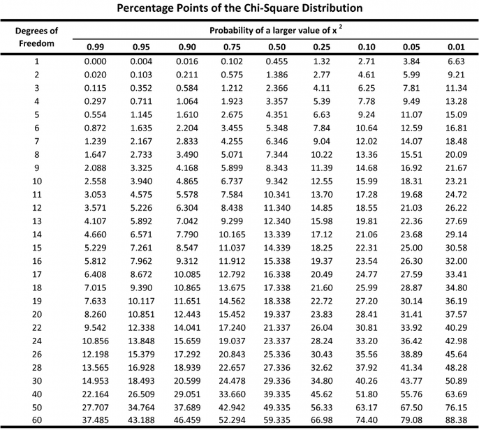
The calculated X2 value is than compared to the “critical value  X2” found in an X2 distribution table.  The X2 distribution table represents a theoretical curve of  expected results. The expected results are based on DEGREES OF  FREEDOM. 

Degrees of Freedom = (number of rows - 1) X (number of columns - 1)
In our example, DF = (2-1) X (2-1) = 1 X 1 = 1
*the row and column for the total in the contingency table are not included
 
The X2 distribution table is organized by the Level of  Significance.  The level of significance is the maximum tolerable probability of accepting a false null hypothesis.  We use 0.05.  ​

• If the calculated value is lower than the critical value in the table at the 0.05 level of significance, accept the null hypothesis and conclude that there is NO significant association between the variables.   

• If the calculated value is higher than the critical value in the table at the 0.05 level of significance, reject the null hypothesis and conclude that there IS a significant association between the variables.  ​

​
For example, with a DF=1, a value greater than 3.841 is required to be considered statistically significant (at p = 0.05). Since the X2 we calculated (0.4) is less than 3.841, there is NOT a significant association between Species A and Species B.  The location of Species A has no significant effect on the location of Species B, any association between species is likely due to chance and sampling error.